
Enumerating structures#
Predicting mixing energies#
In this step the cluster expansion constructed previously will be employed to predict the mixing
energies for a larger set of structures that are obtained by enumeration. After
loading the CE from file, we loop over all structures with up 12 atoms in the
unit cell and compile silver concentrations and predicted mixing energy into a
list, which is calculated by calling the predict method of the ClusterExpansion object with the ASE Atoms object
that represents the present structure as input argument.
ce = ClusterExpansion.read('mixing_energy.ce')
species = ['Ag', 'Pd']
data = {'concentration': [], 'mixing_energy': []}
structures = []
cluster_space = ce.get_cluster_space_copy()
chemical_symbols = cluster_space.chemical_symbols
primitive_structure = cluster_space.primitive_structure
for structure in enumerate_structures(structure=primitive_structure,
                                      sizes=range(1, 13),
                                      chemical_symbols=chemical_symbols):
    conc = structure.symbols.count('Pd') / len(structure)
    data['concentration'].append(conc)
    data['mixing_energy'].append(ce.predict(structure))
    structures.append(structure)
print('Predicted energies for {} structures'.format(len(structures)))
Extracting the convex hull#
Using this set of mixing energies we then generate the convex hull using the
ConvexHull class.
hull = ConvexHull(data['concentration'], data['mixing_energy'])
Plotting the results#
The predicted energies can be plotted together with the convex hull as a function of the concentration.
fig, ax = plt.subplots(figsize=(4, 3))
ax.set_xlabel(r'Pd concentration')
ax.set_ylabel(r'Mixing energy (meV/atom)')
ax.set_xlim([0, 1])
ax.set_ylim([-69, 15])
ax.scatter(data['concentration'], 1e3 * array(data['mixing_energy']),
           marker='x')
ax.plot(hull.concentrations, 1e3 * hull.energies, '-o', color='green')
plt.savefig('mixing_energy_predicted.png', bbox_inches='tight')
The figure thus generated is shown below.
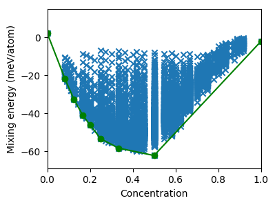
Predicted mixing energies versus concentration for a set of systematically enumerated structures.#
Filtering for low energy structures#
The ConvexHull class also provides some
convenience functions including e.g., the possibility to extract the indices of the
structures that are within a certain distance of the convex hull.
tol = 0.0005
low_energy_structures = hull.extract_low_energy_structures(
    data['concentration'], data['mixing_energy'], tol)
print('Found {} structures within {} meV/atom of the convex hull'.
      format(len(low_energy_structures), 1e3 * tol))
These structures can then be calculated for example using the reference method of choice.
Analyzing stability#
The distance of every structure to the convex hull, commonly referred to as the
energy above the hull, is obtained from get_energy_above_convex_hull. It is zero
for the structures on the hull and positive for all others. The corresponding
boolean mask, which is convenient for filtering a table of results, comes from
is_on_convex_hull.
The remaining functions are built on the facets of the hull, which are the tie
lines of a binary, the three-phase triangles of a ternary, and their analogues
for more species. get_decomposition returns the structures
that a sample of a given overall concentration separates into together with the
fraction of each of them, while get_facets enumerates the coexistence
regions themselves.
The slope of a face is returned by get_facet_gradients, and
get_chemical_potentials turns it into the
chemical potential differences at which the structures on that face coexist.
The two differ whenever a concentration refers to a sublattice rather than to the whole lattice, because the energy of a cluster expansion is given per site of the whole lattice while changing one site changes the concentration of its sublattice by \(1/N_s\). For a system with a single sublattice that covers all sites the two coincide.
get_species_chemical_potentials gives one
chemical potential per species instead of one difference per sublattice, which
is what SemiGrandCanonicalEnsemble takes through its
chemical_potentials argument.
Only differences between species that share a sublattice carry meaning, since those are the exchanges a simulation makes. The species that comes first alphabetically is given a value of zero, and a difference between species of different sublattices is whatever the solution happened to give.
It names species, so it needs a hull that knows which species each
concentration counts. That is a hull built with
from_sublattice_concentrations, which
holds for a system with a single sublattice as much as for one with several.
A hull built by passing concentrations to ConvexHull directly, as above, carries no species and
offers get_chemical_potentials instead:
from icet.tools import (ConvexHull, get_sublattice_concentrations,
                        get_sublattice_site_fractions)

concentrations = get_sublattice_concentrations(structures, cluster_space)
site_fractions = get_sublattice_site_fractions(structures[0], cluster_space)
hull = ConvexHull.from_sublattice_concentrations(
    concentrations, mixing_energies, site_fractions=site_fractions)

for face, potentials in zip(hull.get_facets(),
                            hull.get_species_chemical_potentials()):
    ensemble = SemiGrandCanonicalEnsemble(..., chemical_potentials=potentials)
The result names the species whose concentration varies, and only those. A species held at one composition throughout carries no information for the hull to report, which is the case of a ternary cluster space fed with data along one binary edge, and of a whole sublattice held fixed while another is varied.
A simulation has to leave those species where the hull assumed them.
SemiGrandCanonicalEnsemble holds a whole sublattice fixed
through its sublattice_probabilities argument, and HybridEnsemble holds individual species fixed through the
allowed_symbols of a semi-grand canonical step. Sampling a species that the
result does not name changes a composition the hull took as given, and the
simulation no longer sits at the phase boundary it reports.
A chemical potential belongs to a species and not to a sublattice. When a
species occurs on more than one sublattice, the differences of a face can
constrain the same pair of species twice, and the two constraints need not
agree. Such a face is not a state that a semi-grand canonical simulation can
reach, whatever chemical potentials are chosen, and
get_species_chemical_potentials raises for
it rather than return values that do not describe it. The differences resolved
by sublattice remain available from get_chemical_potentials.
above_hull = hull.get_energy_above_convex_hull(
    data['concentration'], data['mixing_energy'])
print('Largest distance to the convex hull: {:.1f} meV/atom'.
      format(1e3 * max(above_hull)))

# The structures that a given overall concentration separates into, and the
# chemical potential difference at which they coexist, follow from the facets
# of the hull.
decomposition = hull.get_decomposition([0.35])[0]
print('At a Pd concentration of 0.35 the system separates into')
for structure_index, fraction in zip(decomposition['structures'],
                                     decomposition['fractions']):
    concentration = data['concentration'][structure_index]
    print('  {:5.1%} of the structure at a Pd concentration of {:.3f}'.
          format(fraction, concentration))

# Silver and palladium share a single sublattice that covers every site, so the
# chemical potentials coincide with the gradients of the faces here.
for facet, potential in zip(hull.get_facets(), hull.get_chemical_potentials()):
    concentrations = [data['concentration'][i] for i in facet]
    print('Structures at concentrations {} coexist at a chemical potential '
          'difference of {:.1f} meV'.format(
              ['{:.3f}'.format(c) for c in concentrations], 1e3 * potential[0]))
All of these functions work for any number of species and are evaluated for all input concentrations at once.
Systems with several sublattices#
The example above describes the composition with a single concentration, which is all a binary on one sublattice needs. A system with several sublattices, say a metal alloy that also takes up hydrogen on an interstitial sublattice, is described by a concentration on each of them.
get_sublattice_concentrations computes those
concentrations for a set of structures, using the sublattices of the cluster
space, and ConvexHull.from_sublattice_concentrations builds the
hull from them:
from icet.tools import (ConvexHull, get_sublattice_concentrations,
                        get_sublattice_site_fractions)

concentrations = get_sublattice_concentrations(structures, cluster_space)
site_fractions = get_sublattice_site_fractions(structures[0], cluster_space)
hull = ConvexHull.from_sublattice_concentrations(
    concentrations, mixing_energies, site_fractions=site_fractions)
The site fractions are what relate a concentration, which counts one
sublattice, to the energy, which is given per site of the whole lattice. They
are needed by both functions that give chemical potentials, which refuse to
guess them and point at get_sublattice_site_fractions when they are missing.
The geometry of the hull, get_facet_gradients and
get_decomposition included, works without
them.
The concentrations are dictionaries of the form {'A': {'Ag': 0.3, 'Pd':
0.7}, 'B': {'H': 0.2, 'X': 0.8}}, where the keys of the outer dictionary are
the symbols of the sublattices and X denotes a vacancy. Of the species
whose concentration varies on a sublattice the hull needs all but one, since
the others determine it, and a species held at one composition throughout is
left out entirely. concentration_labels records which species
each of them refers to:
>>> hull.concentration_labels
[('A', 'Ag'), ('B', 'H')]
Those labels give the order of the columns of the concentrations, of the target
concentrations passed to the various methods, and of the chemical potentials
returned by get_chemical_potentials. Sublattices that
allow a single species, and species that are held fixed across the whole set of
structures, carry no concentration and are left out.
All structures must share the same underlying lattice, which is the case when they belong to one cluster space. This is what makes the concentration of a mixture of phases the average of their concentrations on every sublattice at once, and hence what makes the hull in this space meaningful.
Source code#
The complete source code is available in
examples/tutorial/3_enumerate_structures.py
# This scripts runs in about 14 minutes on an i7-6700K CPU.

import matplotlib.pyplot as plt
from numpy import array
from icet import ClusterExpansion
from icet.tools import ConvexHull, enumerate_structures

# step 1: Predict energies for enumerated structures
ce = ClusterExpansion.read('mixing_energy.ce')
species = ['Ag', 'Pd']
data = {'concentration': [], 'mixing_energy': []}
structures = []
cluster_space = ce.get_cluster_space_copy()
chemical_symbols = cluster_space.chemical_symbols
primitive_structure = cluster_space.primitive_structure
for structure in enumerate_structures(structure=primitive_structure,
                                      sizes=range(1, 13),
                                      chemical_symbols=chemical_symbols):
    conc = structure.symbols.count('Pd') / len(structure)
    data['concentration'].append(conc)
    data['mixing_energy'].append(ce.predict(structure))
    structures.append(structure)
print('Predicted energies for {} structures'.format(len(structures)))

# step 2: Construct convex hull
hull = ConvexHull(data['concentration'], data['mixing_energy'])

# step 3: Plot the results
fig, ax = plt.subplots(figsize=(4, 3))
ax.set_xlabel(r'Pd concentration')
ax.set_ylabel(r'Mixing energy (meV/atom)')
ax.set_xlim([0, 1])
ax.set_ylim([-69, 15])
ax.scatter(data['concentration'], 1e3 * array(data['mixing_energy']),
           marker='x')
ax.plot(hull.concentrations, 1e3 * hull.energies, '-o', color='green')
plt.savefig('mixing_energy_predicted.png', bbox_inches='tight')

# step 4: Extract candidate ground state structures
tol = 0.0005
low_energy_structures = hull.extract_low_energy_structures(
    data['concentration'], data['mixing_energy'], tol)
print('Found {} structures within {} meV/atom of the convex hull'.
      format(len(low_energy_structures), 1e3 * tol))

# step 5: Analyze the stability of the enumerated structures
above_hull = hull.get_energy_above_convex_hull(
    data['concentration'], data['mixing_energy'])
print('Largest distance to the convex hull: {:.1f} meV/atom'.
      format(1e3 * max(above_hull)))

# The structures that a given overall concentration separates into, and the
# chemical potential difference at which they coexist, follow from the facets
# of the hull.
decomposition = hull.get_decomposition([0.35])[0]
print('At a Pd concentration of 0.35 the system separates into')
for structure_index, fraction in zip(decomposition['structures'],
                                     decomposition['fractions']):
    concentration = data['concentration'][structure_index]
    print('  {:5.1%} of the structure at a Pd concentration of {:.3f}'.
          format(fraction, concentration))

# Silver and palladium share a single sublattice that covers every site, so the
# chemical potentials coincide with the gradients of the faces here.
for facet, potential in zip(hull.get_facets(), hull.get_chemical_potentials()):
    concentrations = [data['concentration'][i] for i in facet]
    print('Structures at concentrations {} coexist at a chemical potential '
          'difference of {:.1f} meV'.format(
              ['{:.3f}'.format(c) for c in concentrations], 1e3 * potential[0]))