Analyzing Monte Carlo simulations
After the Monte Carlo simulations have finished, they can be analyzed in various ways. With dense sampling, it may take several minutes to load the data. It is therefore recommended to first collect all data in averaged form. Here, we read all data containers and take averages but discard data collected during the first five MC cycles to allow for equilibration (please be aware that in general five MC cycles may be insufficient).
for ensemble in ['sgc', 'vcsgc']:
    data = []
    for filename in glob('monte_carlo_data/{}-*.dc'.format(ensemble)):
        dc = DataContainer.read(filename)
        data_row = dc.ensemble_parameters
        data_row['filename'] = filename
        n_atoms = data_row['n_atoms']

        equilibration = 5 * n_atoms

        stats = dc.analyze_data('Pd_count', start=equilibration)
        data_row['Pd_concentration'] = stats['mean'] / n_atoms
        data_row['Pd_concentration_error'] = stats['error_estimate'] / n_atoms

        stats = dc.analyze_data('potential', start=equilibration)
        data_row['mixing_energy'] = stats['mean'] / n_atoms
        data_row['mixing_energy_error'] = stats['error_estimate'] / n_atoms

        data_row['acceptance_ratio'] = \
            dc.get_average('acceptance_ratio', start=equilibration)
        if ensemble == 'sgc':
            data_row['free_energy_derivative'] = \
                dc.ensemble_parameters['mu_Pd'] - \
                dc.ensemble_parameters['mu_Ag']
        elif ensemble == 'vcsgc':
            data_row['free_energy_derivative'] = \
                dc.get_average('free_energy_derivative_Pd', start=equilibration)

        data.append(data_row)
Next, we create a pandas DataFrame object which we store as a csv-file for future access.
    df = pd.DataFrame(data)
    df.to_csv('monte-carlo-{}.csv'.format(ensemble), sep='\t')
Now, we can easily and quickly load the aggregated data and inspect properties of interest, such as the free energy derivative as a function of concentration.
dfs = {}
dfs['sgc'] = pd.read_csv('monte-carlo-sgc.csv', delimiter='\t')
dfs['vcsgc'] = pd.read_csv('monte-carlo-vcsgc.csv', delimiter='\t')


# step 1: Plot free energy derivatives
colors = {300: '#D62728',  # red
          900: '#1F77B4'}  # blue
linewidths = {'sgc': 3, 'vcsgc': 1}
alphas = {'sgc': 0.5, 'vcsgc': 1.0}
fig, ax = plt.subplots(figsize=(4, 3.5))
for ensemble, df in dfs.items():
    for T in sorted(df.temperature.unique()):
        df_T = df.loc[df['temperature'] == T].sort_values('Pd_concentration')
        ax.plot(df_T['Pd_concentration'],
                1e3 * df_T['free_energy_derivative'],
                marker='o', markersize=2.5,
                label='{}, {} K'.format(ensemble, T),
                color=colors[T],
                linewidth=linewidths[ensemble], alpha=alphas[ensemble])
ax.set_xlabel('Pd concentration')
ax.set_ylabel('Free energy derivative (meV/atom)')
ax.set_xlim([-0.02, 1.02])
ax.set_ylim([-600, 500])
ax.legend()
plt.savefig('free_energy_derivative.png', bbox_inches='tight')
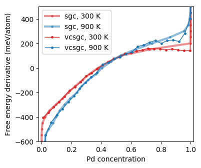
Free energy derivative as a function of concentration from Monte Carlo simulations in the semi-grand canonical (SGC) and variance-constrained semi-grand canonical (VCSGC) ensembles (the curves are noisy due to insufficient sampling).
A gap in the semi-grand canonical (SGC) data around 85% Pd indicates a very asymmetric miscibility gap, which agrees with previous assessments of the phase diagram. It is possible to sample across the miscibility gap using the variance-constrained semi-grand canonical (VCSGC) ensemble for sampling. The latter, however, might require longer simulation times to obtain well converged data.
It can also be instructive to plot the mixing energy.
df = dfs['sgc']
fig, ax = plt.subplots(figsize=(4, 3.5))
for T in sorted(df.temperature.unique()):
    df_T = df.loc[df['temperature'] == T].sort_values('Pd_concentration')
    e_mix = 1e3 * df_T['mixing_energy']
    e_mix_error = 1e3 * df_T['mixing_energy_error']
    ax.plot(df_T['Pd_concentration'], e_mix,
            marker='o', markersize=2.5, label='{} K'.format(T),
            color=colors[T])
    # Plot error estimate
    ax.fill_between(df_T['Pd_concentration'],
                    e_mix + e_mix_error, e_mix - e_mix_error,
                    color=colors[T], alpha=0.4)
ax.set_xlabel('Pd concentration')
ax.set_ylabel('Mixing energy (meV/atom)')
ax.set_xlim([-0.02, 1.02])
ax.legend()
plt.savefig('mixing_energy_sgc.png', bbox_inches='tight')
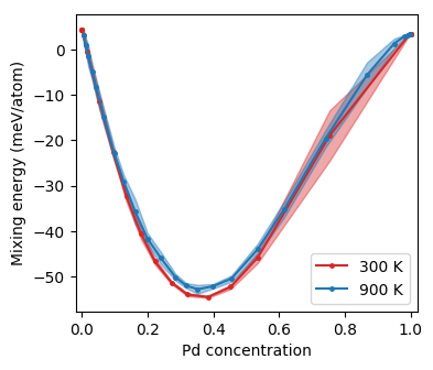
Mixing energy as a function of concentration from Monte Carlo simulations in the SGC ensemble.
Furthermore one might want to consider for example the acceptance ratio.
df = dfs['sgc']
fig, ax = plt.subplots(figsize=(4, 3.5))
for T in sorted(df.temperature.unique()):
    df_T = df.loc[df['temperature'] == T].sort_values('Pd_concentration')
    ax.plot(df_T['Pd_concentration'], df_T['acceptance_ratio'],
            marker='o', markersize=2.5, label='{} K'.format(T),
            color=colors[T])
ax.set_xlabel('Pd concentration')
ax.set_ylabel('Acceptance ratio')
ax.set_xlim([-0.02, 1.02])
ax.legend()
plt.savefig('acceptance_ratio_sgc.png', bbox_inches='tight')
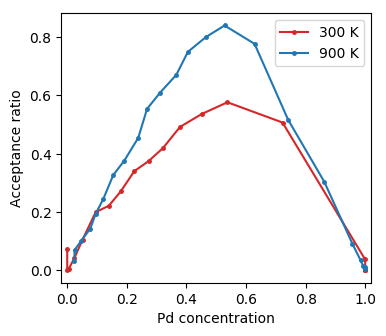
Acceptance ratio as a function of concentration from Monte Carlo simulations in the SGC ensemble.
As expected the acceptance ratio increases with temperature and is maximal for intermediate concentrations.
Source code
The source code for data aggregation is available in
examples/tutorial/6_analyze_monte_carlo.py.
import pandas as pd
from glob import glob
from mchammer import DataContainer

# step 1: Collect data from SGC and VCSGC simulations
for ensemble in ['sgc', 'vcsgc']:
    data = []
    for filename in glob('monte_carlo_data/{}-*.dc'.format(ensemble)):
        dc = DataContainer.read(filename)
        data_row = dc.ensemble_parameters
        data_row['filename'] = filename
        n_atoms = data_row['n_atoms']

        equilibration = 5 * n_atoms

        stats = dc.analyze_data('Pd_count', start=equilibration)
        data_row['Pd_concentration'] = stats['mean'] / n_atoms
        data_row['Pd_concentration_error'] = stats['error_estimate'] / n_atoms

        stats = dc.analyze_data('potential', start=equilibration)
        data_row['mixing_energy'] = stats['mean'] / n_atoms
        data_row['mixing_energy_error'] = stats['error_estimate'] / n_atoms

        data_row['acceptance_ratio'] = \
            dc.get_average('acceptance_ratio', start=equilibration)
        if ensemble == 'sgc':
            data_row['free_energy_derivative'] = \
                dc.ensemble_parameters['mu_Pd'] - \
                dc.ensemble_parameters['mu_Ag']
        elif ensemble == 'vcsgc':
            data_row['free_energy_derivative'] = \
                dc.get_average('free_energy_derivative_Pd', start=equilibration)

        data.append(data_row)

    # step 2: Write data to pandas dataframe in csv format
    df = pd.DataFrame(data)
    df.to_csv('monte-carlo-{}.csv'.format(ensemble), sep='\t')
The source code for generating the figures is available in
examples/tutorial/7_plot_monte_carlo_data.py.
import matplotlib.pyplot as plt
import pandas as pd

# step 1: Load data frame
dfs = {}
dfs['sgc'] = pd.read_csv('monte-carlo-sgc.csv', delimiter='\t')
dfs['vcsgc'] = pd.read_csv('monte-carlo-vcsgc.csv', delimiter='\t')


# step 1: Plot free energy derivatives
colors = {300: '#D62728',  # red
          900: '#1F77B4'}  # blue
linewidths = {'sgc': 3, 'vcsgc': 1}
alphas = {'sgc': 0.5, 'vcsgc': 1.0}
fig, ax = plt.subplots(figsize=(4, 3.5))
for ensemble, df in dfs.items():
    for T in sorted(df.temperature.unique()):
        df_T = df.loc[df['temperature'] == T].sort_values('Pd_concentration')
        ax.plot(df_T['Pd_concentration'],
                1e3 * df_T['free_energy_derivative'],
                marker='o', markersize=2.5,
                label='{}, {} K'.format(ensemble, T),
                color=colors[T],
                linewidth=linewidths[ensemble], alpha=alphas[ensemble])
ax.set_xlabel('Pd concentration')
ax.set_ylabel('Free energy derivative (meV/atom)')
ax.set_xlim([-0.02, 1.02])
ax.set_ylim([-600, 500])
ax.legend()
plt.savefig('free_energy_derivative.png', bbox_inches='tight')

# step 2: Plot mixing energy vs composition
df = dfs['sgc']
fig, ax = plt.subplots(figsize=(4, 3.5))
for T in sorted(df.temperature.unique()):
    df_T = df.loc[df['temperature'] == T].sort_values('Pd_concentration')
    e_mix = 1e3 * df_T['mixing_energy']
    e_mix_error = 1e3 * df_T['mixing_energy_error']
    ax.plot(df_T['Pd_concentration'], e_mix,
            marker='o', markersize=2.5, label='{} K'.format(T),
            color=colors[T])
    # Plot error estimate
    ax.fill_between(df_T['Pd_concentration'],
                    e_mix + e_mix_error, e_mix - e_mix_error,
                    color=colors[T], alpha=0.4)
ax.set_xlabel('Pd concentration')
ax.set_ylabel('Mixing energy (meV/atom)')
ax.set_xlim([-0.02, 1.02])
ax.legend()
plt.savefig('mixing_energy_sgc.png', bbox_inches='tight')

# step 3: Plot acceptance ratio vs composition
df = dfs['sgc']
fig, ax = plt.subplots(figsize=(4, 3.5))
for T in sorted(df.temperature.unique()):
    df_T = df.loc[df['temperature'] == T].sort_values('Pd_concentration')
    ax.plot(df_T['Pd_concentration'], df_T['acceptance_ratio'],
            marker='o', markersize=2.5, label='{} K'.format(T),
            color=colors[T])
ax.set_xlabel('Pd concentration')
ax.set_ylabel('Acceptance ratio')
ax.set_xlim([-0.02, 1.02])
ax.legend()
plt.savefig('acceptance_ratio_sgc.png', bbox_inches='tight')