Comparison with target data
In this step the performance of the cluster expansion constructed in the
previous step will be tested
against the target data. After loading the CE from file, we loop over all
configurations in the database of reference structure and compile the
concentration as well as the target and predicted mixing energies into a
dictionary. Note that the latter of the three values is calculated by calling
the predict() method of the
ClusterExpansion object with the ASE
Atoms object that represents the present structure as input
argument.
ce = ClusterExpansion.read('mixing_energy.ce')
data = {'concentration': [], 'reference_energy': [], 'predicted_energy': []}
db = connect('reference_data.db')
for row in db.select('natoms<=6'):
    data['concentration'].append(row.concentration)
    # the factor of 1e3 serves to convert from eV/atom to meV/atom
    data['reference_energy'].append(1e3 * row.mixing_energy)
    data['predicted_energy'].append(1e3 * ce.predict(row.toatoms()))
Once this step has completed the predicted and target mixing energies are plotted as functions of the concentration.
fig, ax = plt.subplots(figsize=(4, 3))
ax.set_xlabel(r'Pd concentration')
ax.set_ylabel(r'Mixing energy (meV/atom)')
ax.set_xlim([0, 1])
ax.set_ylim([-69, 15])
ax.scatter(data['concentration'], data['reference_energy'],
           marker='o', label='reference')
ax.scatter(data['concentration'], data['predicted_energy'],
           marker='x', label='CE prediction')
plt.savefig('mixing_energy_comparison.png', bbox_inches='tight')
The figure generated by this diagram is shown below.
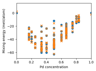
Predicted (orange crosses) and target (blue circles) mixing energies versus concentration for the structures used in the construction of the cluster expansion.
Source code
The complete source code is available in
examples/tutorial/2_compare_to_target_data.py
# This scripts runs in about 6 seconds on an i7-6700K CPU.

import matplotlib.pyplot as plt
from ase.db import connect
from icet import ClusterExpansion

# step 1: Compile predicted and reference data for plotting
ce = ClusterExpansion.read('mixing_energy.ce')
data = {'concentration': [], 'reference_energy': [], 'predicted_energy': []}
db = connect('reference_data.db')
for row in db.select('natoms<=6'):
    data['concentration'].append(row.concentration)
    # the factor of 1e3 serves to convert from eV/atom to meV/atom
    data['reference_energy'].append(1e3 * row.mixing_energy)
    data['predicted_energy'].append(1e3 * ce.predict(row.toatoms()))

# step 2: Plot results
fig, ax = plt.subplots(figsize=(4, 3))
ax.set_xlabel(r'Pd concentration')
ax.set_ylabel(r'Mixing energy (meV/atom)')
ax.set_xlim([0, 1])
ax.set_ylim([-69, 15])
ax.scatter(data['concentration'], data['reference_energy'],
           marker='o', label='reference')
ax.scatter(data['concentration'], data['predicted_energy'],
           marker='x', label='CE prediction')
plt.savefig('mixing_energy_comparison.png', bbox_inches='tight')